[Alicia Calafat, Joan-Rene Merou, Sheila Dwyer, Robert Schofield, Jenne Driggers]



Scope
We analyze violin harmonics and their intermodulation products in H1:OMC-DCPD_SUM_OUT_DQ, and estimate the quadratic mixing coefficient β for those products. Peak detection and confirmation use an Ansel-inspired adaptive-threshold approach on a stabilized series, combined with simple height floors. We then confirm analytically expected intermodulation frequencies and compute beta from amplitude products of paired parent lines and their intermodulation.



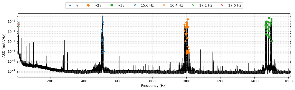
Calibration lines at 15.6, 16.4, 17.1, and 17.6 Hz:







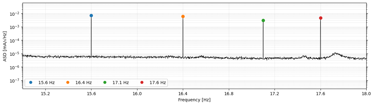
The full-band ASD (about 10 to 1610 Hz) shows violin harmonics near 500 Hz (v), about 1000 Hz (2v), and about 1500 Hz (3v), together with the labeled calibration tones. This context motivates the intermodulation search at violin plus/minus calibration, and at violin-violin sums and differences across the band.







Problem and physical context
Small-signal readout model (mA domain, OUT):

y(t) = α s(t) + β s(t)^2

where s(t) is the photocurrent at DCPD SUM (mA), α is the linear gain, and β is the weak quadratic nonlinearity coefficient (mA-1).

Single violin tone at fv and calibration tone at fcal:

s(t) = X sin(2 π fv t) + Z sin(2 π fcal t)

Square s(t):

s(t)^2 = X^2 sin^2(2 π fv t) + Z^2 sin^2(2 π fcal t) + 2 X Z sin(2 π fv t) sin(2 π fcal t)

Use identities:

sin^2(u) = (1 - cos(2u)) / 2    2 sin(a) sin(b) = cos(a - b) - cos(a + b)

Decomposition

  - Self terms:

    X^2 sin^2(2 π fv t) → DC and a line at 2 fv.

    Z^2 sin^2(2 π fcal t) → DC and a line at 2 fcal.

    - We ignore DC (0 Hz).

    - The 2 fv component is used inside the violin–violin families as the i = j "sum" case (often labeled vv_h2). Estimator: βself(v) = A2v / (Av Av).

    - The 2 fcal component is not used for β (no "cal–cal" family here), though it may be visible.

  - Cross term (interaction):

    2 X Z sin(2 π fv t) sin(2 π fcal t) = X Z [ cos(2 π (fv - fcal) t) - cos(2 π (fv + fcal) t) ] → mixing lines at fv ± fcal with amplitudes ∝ β X Z.

Spectral amplitudes from PSD (same convention for all lines)

PSD has units mA2/Hz. Let Δf be the bin width. For a narrow line:

Abin(f) = sqrt(PSD(f) · Δf) = ASD(f) · sqrt(Δf) [mA].

For robustness we integrate ± 1 bin around the peak index:

Abin ≈ sqrt((PSD[i-1] + PSD[i] + PSD[i+1]) · Δf).

Quadratic mixing scaling used for the estimator:

Amix ∝ β · AL · AR.

Per-line β estimators used here:

  - Violin ± calibration:

    β = A(v±cal) / (Av Acal) [mA-1].

  - Violin self-mix (i = j) at 2 fv (vv_h2):

    βself(v) = A2v / (Av Av) [mA-1].

  - General violin–violin (i ≠ j) sums/diffs:

    β = A(f_i±f_j) / (Af_i Af_j) [mA-1].



How the scripts work
  - Intermodulation explorer: input long spectrum (f, PSD); derive ASD; estimate band medians; detect violin peaks with an adaptive threshold on a stabilized series plus simple height floors; propose and confirm intermods at violin ± calibration and violin–violin sums/diffs; export plots and a JSON summary.

  - Beta estimator: read the JSON and the same spectrum; reconstruct A_left, A_right, A_mix via ± 1-bin PSD integration; compute beta_hat = A_mix_bin / (A_left_bin · A_right_bin); summarize by families and produce plots.



Current intermodulation detections
These are the retained detections after applying our thresholds and pairing rules. They are the inputs used downstream to compute and summarize beta by family.

  - Detected violin peaks kept: v = 20, approx 2v = 25, approx 3v = 30.

  - Intermod candidates before pairing: v plus/minus cal total = 154; violin–violin (sums and differences) total = 761.

  - Paired intermods kept for beta: v plus/minus cal = 22; 2v plus/minus cal = 18; 3v plus/minus cal = 18; vv(fund) = 386; vv(2v) = 247; vv(3v) = 128.



Beta results (paired families)

  

    

      
Family
      
Paired count
      
beta median [1/mA]
    
  
  

    
v ± cal
22
0.638
    
2v ± cal
18
0.450
    
3v ± cal
18
0.286
    
vv (fund)
386
10.824
    
vv (2v)
247
1.586
    
vv (3v)
128
13.329
  




Plots

1) Calibration-violin explorer


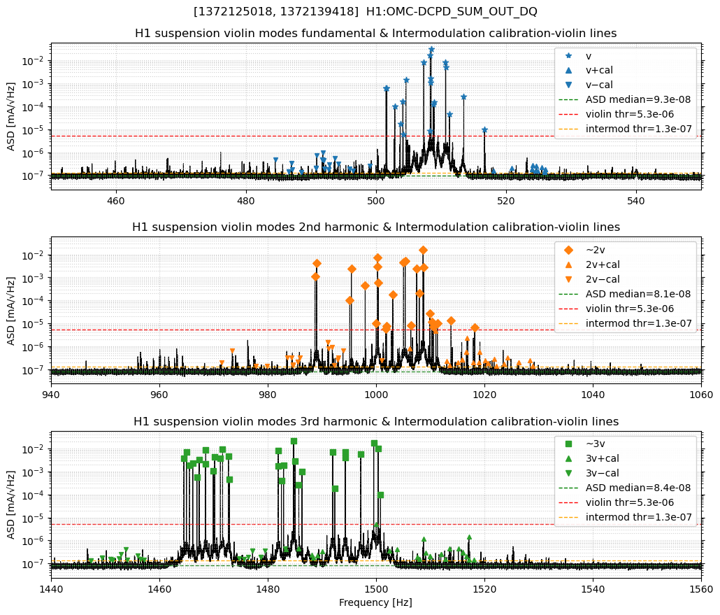
Calibration tones align as symmetric sidebands around violin harmonics at the predicted offsets (v ± fcal). This validates the pairing rules used for beta estimation and shows that v ± cal families are present at v, 2v, and 3v.

2) Violin-violin explorer


Sums and differences of violin peaks form dense loci at the predicted frequencies. Violin-violin intermods are abundant in all three bands.


Meaning of "violin–violin": all sum/difference pairings between detected harmonics (v, 2v, 3v), both same-harmonic and cross-harmonic, are tested as (fi + fj) and abs(fi - fj) (i.e., v+v and abs(v-v), 2v+2v and abs(2v-2v), 3v+3v and abs(3v-3v), v+2v and abs(v-2v), v+3v and abs(v-3v), 2v+3v and abs(2v-3v)); only those landing in the displayed band are plotted.

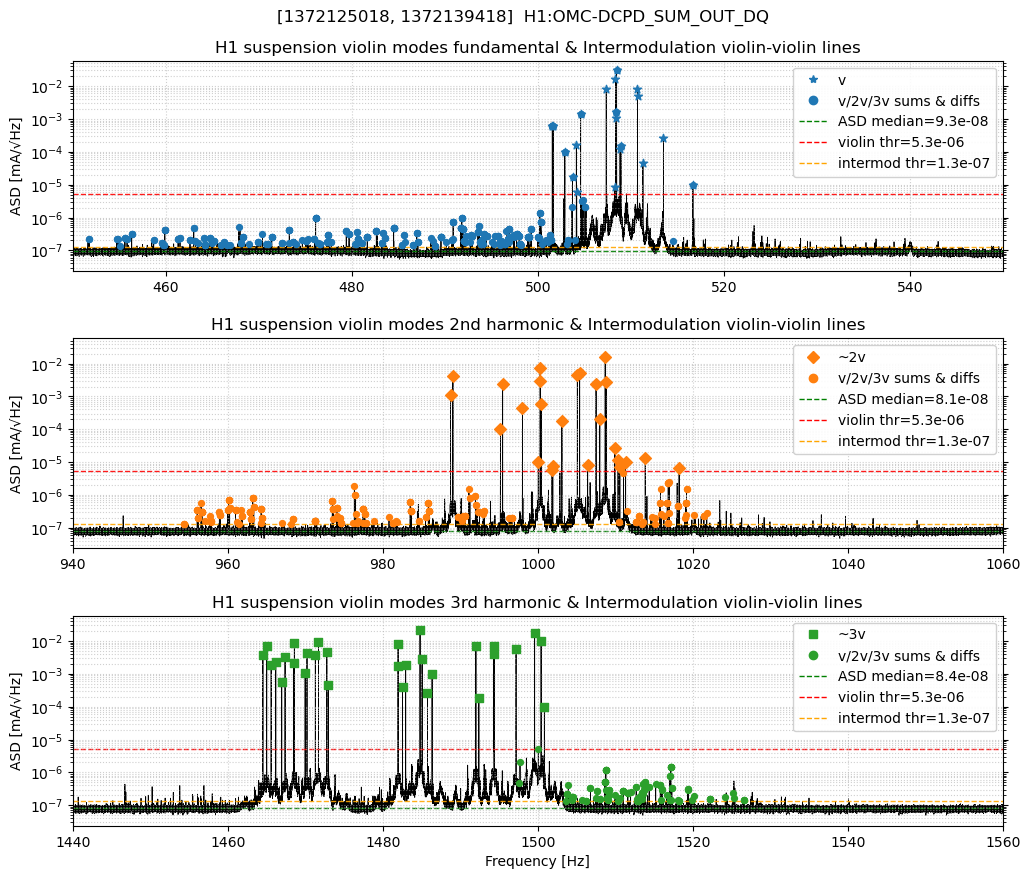
3) Violin and intermods (zoom panels with thresholds)


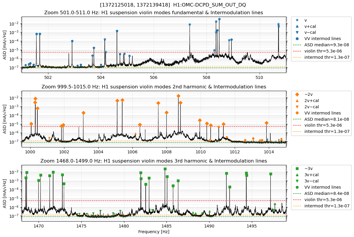
Zooms around about 500, about 1000, and about 1490 Hz show violin peaks, calibration sidebands, and violin-violin intermods. Thresholds used (representative):

  - Band medians (ASD): about 9.29e-08 (v), 8.12e-08 (2v), 8.38e-08 (3v).

  - Violin peak floor (ASD): about 5.3e-06.

  - Intermod minimum height (ASD): about 1.3e-07.

Adaptive selection tracks local noise; loosening/tightening these settings trades recall vs precision. The chosen values recover the strong violins and yield a physically plausible intermod count for stable beta.

4) Beta histograms by family


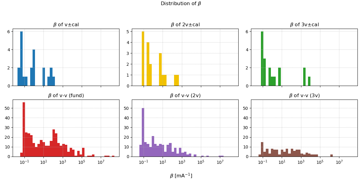
Violin-violin families peak at larger beta than calibration mixes, as expected for a quadratic mechanism scaling with the product of parent amplitudes. Broader tails appear near thresholds and in crowded regions.

5) Beta by intermodulation family


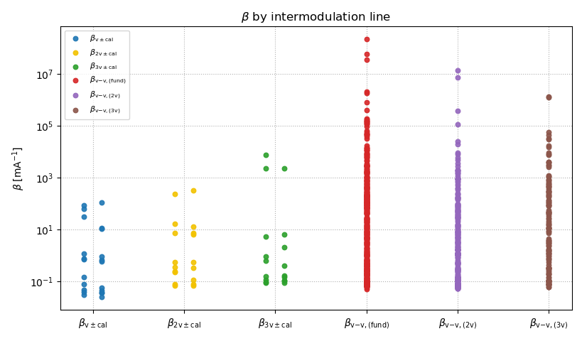
The hierarchy is clear: vv(fund) and vv(3v) give the largest medians; vv(2v) is smaller but still above all calibration mixes. This is consistent with larger and cleaner A_left x A_right for violin–violin pairs than for violin ± calibration.

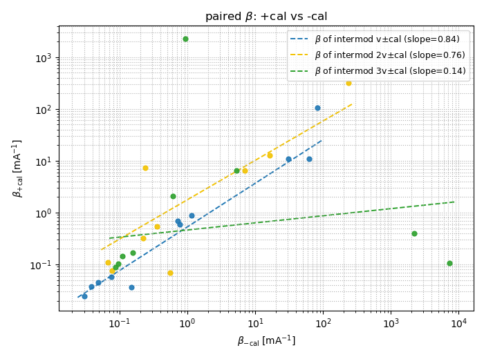
6) β(+cal) versus β(-cal)


v and 2v show near-diagonal symmetry; 3v is imbalanced, consistent with leakage or pairing sensitivity at the third harmonic.

7) Amix versus (AL · AR) - quadratic check


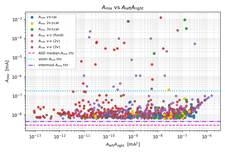
Largest deviations sit near thresholds and in crowded sub-bands.

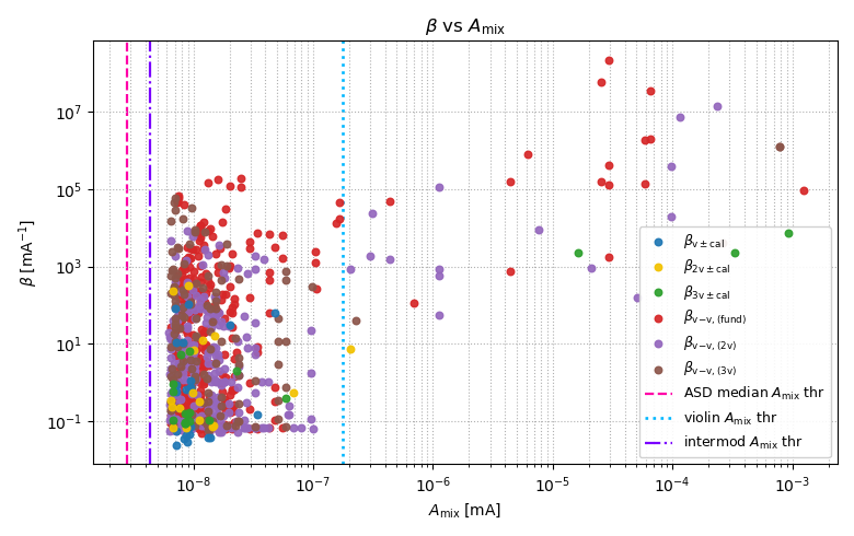
8) β versus Amix with thresholds


Scatter grows as Amix approaches thresholds.



Next steps
  - Repeat the analysis in the ADC domain (counts) for H1:OMC-DCPD_SUM_IN. Use the OMC_DCPD filter magnitude file (cols: freq, DCPD A mag, DCPD B mag) to convert counts<->mA and recompute beta. Comparing OUT (mA) and IN (counts) will test for any domain-dependent bias in beta.